다층 퍼셉트론 신경망 모델 구현

피마족 인디언 당뇨병 발병 데이터셋(이진 클래스 문제)

전체코드

import numpy as np
from keras.models import Sequential
from keras.layers import Dense
import pandas as pd
from sklearn.model_selection import train_test_split

# 랜덤 시드 고정시키기
np.random.seed(5)

# 1. 데이터 준비
dataset = pd.read_csv('/content/pima-indians-diabetes.csv')
X = dataset.iloc[:,0:8].values
y = dataset.iloc[:,8].values

# 2. 데이터 분리
X_train, X_test, y_train, y_test = train_test_split(X,y,test_size = 0.2 )

# 3. 모델 구성하기
model = Sequential()
model.add(Dense(12, input_dim=8, activation='relu'))
model.add(Dense(8, activation='relu'))
model.add(Dense(1, activation='sigmoid'))

# 4. 모델 학습과정 설정하기
model.compile(loss='binary_crossentropy', optimizer = 'adam', metrics=['accuracy'])

# 5. 모델 학습시키기
model.fit(X_train, y_train, epochs= 1500, batch_size = 94)

# 6. 모델 평가하기
score = model.evaluate(X_test, y_test)
print(score)

Epoch 1/1500
7/7 [==============================] - 0s 3ms/step - loss: 7.0155 - accuracy: 0.6515
Epoch 2/1500
7/7 [==============================] - 0s 3ms/step - loss: 5.5714 - accuracy: 0.6515
...
...
...
Epoch 1499/1500
7/7 [==============================] - 0s 3ms/step - loss: 0.4390 - accuracy: 0.7850
Epoch 1500/1500
7/7 [==============================] - 0s 3ms/step - loss: 0.4393 - accuracy: 0.7915
5/5 [==============================] - 0s 3ms/step - loss: 0.4591 - accuracy: 0.7727
[0.45910510420799255, 0.7727272510528564]

의류 이미지 분류

패션 MNIST 데이터셋

전체코드

import tensorflow as tf
import numpy as np
import matplotlib.pyplot as plt

#패션 MNIST 데이터셋
fashion_mnist = tf.keras.datasets.fashion_mnist

#데이터 나누기
(train_images, train_labels), (test_images, test_labels) = fashion_mnist.load_data()

class_names = ['T-shirt/top', 'Trouser', 'Pullover', 'Dress', 'Coat',
               'Sandal', 'Shirt', 'Sneaker', 'Bag', 'Ankle boot']

#image의 범위가 0~255이므로 0~1 로 조정
train_images = train_images / 255.0
test_images = test_images / 255.0

#모델 층 설정
model = tf.keras.Sequential([
    tf.keras.layers.Flatten(input_shape=(28, 28)),
    tf.keras.layers.Dense(128, activation='relu'),
    tf.keras.layers.Dense(10)
])

#모델 학습과정 설정(모델 컴파일)
model.compile(optimizer='adam',
              loss=tf.keras.losses.SparseCategoricalCrossentropy(from_logits=True),
              metrics=['accuracy'])

#모델 학습(모델 fit)
model.fit(train_images, train_labels, epochs=10)

#정확도 평가
test_loss, test_acc = model.evaluate(test_images,  test_labels, verbose=2)

print('\nTest accuracy:', test_acc)

Epoch 1/10
1875/1875 [==============================] - 5s 2ms/step - loss: 0.5011 - accuracy: 0.8249
...
...
Epoch 9/10
1875/1875 [==============================] - 5s 3ms/step - loss: 0.2472 - accuracy: 0.9076
Epoch 10/10
1875/1875 [==============================] - 4s 2ms/step - loss: 0.2405 - accuracy: 0.9104
313/313 - 0s - loss: 0.3293 - accuracy: 0.8868 - 485ms/epoch - 2ms/step

Test accuracy: 0.8867999911308289

예측

#예측 모델의 객체 생성
probability_model = tf.keras.Sequential([model, tf.keras.layers.Softmax()])

#테스트이미지 예측
predictions = probability_model.predict(test_images)

#예측된 값을 시각화 하기위한 함수들
def plot_image(i, predictions_array, true_label, img):
  true_label, img = true_label[i], img[i]
  plt.grid(False)
  plt.xticks([])
  plt.yticks([])

  plt.imshow(img, cmap=plt.cm.binary)

  predicted_label = np.argmax(predictions_array)
  if predicted_label == true_label:
    color = 'blue'
  else:
    color = 'red'

  plt.xlabel("{} {:2.0f}% ({})".format(class_names[predicted_label],
                                100*np.max(predictions_array),
                                class_names[true_label]),
                                color=color)

def plot_value_array(i, predictions_array, true_label):
  true_label = true_label[i]
  plt.grid(False)
  plt.xticks(range(10))
  plt.yticks([])
  thisplot = plt.bar(range(10), predictions_array, color="#777777")
  plt.ylim([0, 1])
  predicted_label = np.argmax(predictions_array)

  thisplot[predicted_label].set_color('red')
  thisplot[true_label].set_color('blue')

예측된 15개의 데이터 시각화

num_rows = 5
num_cols = 3
num_images = num_rows*num_cols
plt.figure(figsize=(2*2*num_cols, 2*num_rows))
for i in range(num_images):
  plt.subplot(num_rows, 2*num_cols, 2*i+1)
  plot_image(i, predictions[i], test_labels, test_images)
  plt.subplot(num_rows, 2*num_cols, 2*i+2)
  plot_value_array(i, predictions[i], test_labels)
plt.tight_layout()
plt.show()

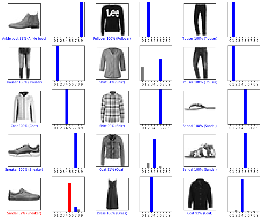
12번째 데이터 불일치!!

---

학습으로 배운점

모델 학습 단계

1. 데이터 전처리 및 준비
2. 데이터셋 생성 과 훈련세트, 테스트세트 분리
3. 모델 구성
4. 모델 학습과정 설정(모델 컴파일)
5. 모델 학습
6. 모델 평가
7. 모델 예측

레이어

• Flatten Layer : 1차원이 아닌 데이터를 1차원으로 변환하여 주는 레이어(주로 이미지 학습때 입력 레이어로 많이 사용)
• Dense Layer : 입력 뉴런 수에 상관없이 출력 뉴런수를 자유롭게 설정할 수 있는 레이어

활성화 함수(activation)

• Sigmoid : 계산한값이 0과 1사이로 표현할 때 사용
• Relu : 계산값이 양수일때 사용
• softmax : 다중 클래스분류 문제에서 출력층에 주로 사용

최적화 함수(optimizer)

• adam : 경사 하강법 알고리즘 중 하나

손실 함수(loss)

• binary_crossentropy : 이진 클래스 문제에 사용
• CategoricalCrossentropy : 레이블과 예측 간의 교차 엔트로피 손실을 계산

기타

• matplot 사용법