비지도 학습(K-means 실습)

• 종속변수가 없는 즉, 정답이 없는 비지도 학습
• 데이터의 유의미한 패턴 / 구조 발견

---

군집화(Clustering)

유사한 특징을 가지는 데이터들의 그룹화
Classification != Clustering

---

K-means(K-평균)

데이터를 K 개의 클러스터(그룹)로 군집화하는 알고리즘,
각 데이터로부터 이들이 속한 클러스터의 중심점(Centroid) 까지의 평균 거리 계산

K-means 동작 순서

1. K 값 설정
2. 지정된 K 개 만큼의 랜덤 좌표 설정
3. 모든 데이터로부터 가장 가까운 중심점 선택
4. 데이터들의 평균 중심으로 중심점 이동
5. 중심점이 더 이상 이동되지 않을 때까지 반복

---

K-means의 한계

시작 점이 랜덤 좌표로 설정 되기 때문에 최종 군집화 모양이 제 각각인 경우가 흔함

K-means++

K-means의 한계를 보완하기 위해 랜덤으로 선정된 시작지점에서 제일먼 데이터를 다음 중심점으로 선정

---

최적의 K를 구하는법

Elbow Method(엘보우 방법)

---

K-Means 실습

import numpy as np
import matplotlib.pyplot as plt
import pandas as pd

dataset = pd.read_csv('..\PythonMLWorkspace(LightWeight)\ScikitLearn\KMeansData.csv')

비지도 학습은 정답인 종속변수가 없기 때문에 y값은 따로 안 정해준다

X = dataset.iloc[:, :].values
# X = dataset.values
# X = dataset.to_numpy() # 공식 홈페이지 권장 방식
X[:5]

array([[ 7.33, 73.  ],
       [ 3.71, 55.  ],
       [ 3.43, 55.  ],
       [ 3.06, 89.  ],
       [ 3.33, 79.  ]])

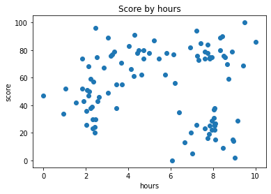
데이터 시각화(전체 데이터 분포 확인)

plt.scatter(X[:, 0], X[:,1]) #축 : hour, y축 :score
plt.title('Score by hours')
plt.xlabel('hours')
plt.ylabel('score')
plt.ylabel('score')

Text(0, 0.5, 'score')

​

데이터 시각화 (축 범위 통일)
축과 축이 서로 단위가 다르면 거리 측정에 오류가 생김

plt.scatter(X[:, 0], X[:,1]) #축 : hour, y축 :score
plt.title('Score by hours')
plt.xlabel('hours')
plt.xlim(0,100)
plt.ylabel('score')
plt.ylim(0,100)
plt.ylabel('score')

Text(0, 0.5, 'score')

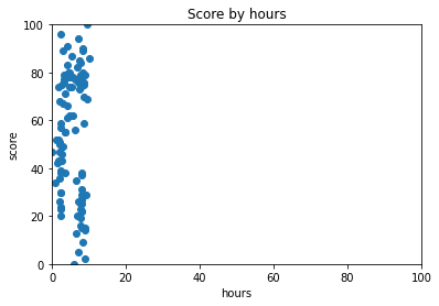
위와 같이 X축을 100가지 늘려주면 가독성이 떨어짐

피쳐 스케일링 (Feature Scaling)

from sklearn.preprocessing import StandardScaler
sc = StandardScaler()
X = sc.fit_transform(X)
X[:5]

array([[ 0.68729921,  0.73538376],
       [-0.66687438,  0.04198891],
       [-0.77161709,  0.04198891],
       [-0.9100271 ,  1.35173473],
       [-0.8090252 ,  0.96651537]])

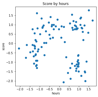
데이터 시각화 (스케일링 데이터)

plt.figure(figsize=(5,5)) # 5X5로 그래프를 맞추기
plt.scatter(X[:, 0], X[:,1]) #축 : hour, y축 :score
plt.title('Score by hours')
plt.xlabel('hours')
plt.ylabel('score')
plt.ylabel('score')

​

​

최적의 K값 찾기(Elbow Method)

inertia : 각 지점부터 클러스터의 중심까지의 거리의 제곱의 합

from sklearn.cluster import KMeans
inertia_list = [] #Cluster에 속한 데이터가 얼마나 가깝게 모여있나.
for i in range(1,11):
    kmeans = KMeans(n_clusters=i, init='k-means++',random_state=0)
    kmeans.fit(X)
    inertia_list.append(kmeans.inertia_) #각 지점으로부터 클러스터의 중심까지의 거리의 제곱의 합

plt.plot(range(1,11),inertia_list)
plt.title("Elbow Method")
plt.xlabel('n_clusters')
plt.ylabel('interia')
plt.show()

​ ​

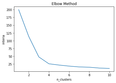
최적의 K(4) 값으로 KMeans 학습

K = 4 # 최적의 K 값
kmeans = KMeans(n_clusters=K, random_state = 0)
#kmeans.fit(X)
y_kmeans = kmeans.fit_predict(X)

데이터 시각화 (최적의 K)

for cluster in range(K):
    plt.scatter(X[y_kmeans == cluster, 0],X[y_kmeans == cluster, 1],s=100, edgecolors='black')
    plt.scatter(kmeans.cluster_centers_[cluster,0], centers[cluster,1],s=300, edgecolor='black',color='yellow',marker='s')
    plt.text(kmeans.cluster_centers_[cluster,0], centers[cluster,1], cluster, va='center', ha='center') #클러스터 텍스트 출력

plt.title('Score by hours')
plt.xlabel('hours')
plt.ylabel('score')
plt.show()

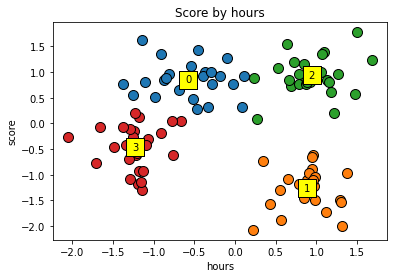
클러스터의 중심의 좌표

centers = kmeans.cluster_centers_
print(centers)

[[-0.57163957  0.85415973]
 [ 0.8837666  -1.26929779]
 [ 0.94107583  0.93569782]
 [-1.22698889 -0.46768593]]

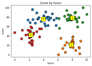
데이터 시각화(스케일링 원상복구)

X_org = sc.inverse_transform(X) # Feature Scaling 된 데이터를 다시 원복
centers_org = sc.inverse_transform(centers)

for cluster in range(K):
    plt.scatter(X_org[y_kmeans == cluster, 0],X_org[y_kmeans == cluster, 1],s=100, edgecolors='black')
    plt.scatter(centers_org[cluster,0], centers_org[cluster,1],s=300, edgecolor='black',color='yellow',marker='s')
    plt.text(centers_org[cluster,0], centers_org[cluster,1], cluster, va='center', ha='center') #클러스터 텍스트 출력

plt.title('Score by hours')
plt.xlabel('hours')
plt.ylabel('score')
plt.show()

​ ​